Table of Contents
- About
- Inputs and Outputs
- Running
- Program Architecture
- How Can I Contribute?
- Config / YAML Information
- Known Issues
- Contributors
- Further Acknowledgements
About
Shear Optimization with ShOpt.jl, a julia library for empirical point spread function characterizations. We aim to improve upon the current state of Point Spread Function Modeling by using Julia to leverage performance gains, use a different mathematical formulation than the literature to provide more robust analytic and pixel grid fits, improve the diagnostic plots, and add features such as wavelets and shapelets. At this projects conclusion we will compare to existing software such as PIFF and PSFex. Work done under McCleary’s Group.
We release the related benchmarking code at https://github.com/mcclearyj/cweb_psf
Start by Cloning This Repository. Then see TutorialNotebook.ipynb or follow along the rest of this README.md to get started! Note that the commands in the tutorial notebook are meant to give a sense of procedure and can be executed with the Julia REPL itself.
Who Should Use
Users looking for empirical point spread function characterization software tailored for the data coming from the James Webb Space Telescope, or on a dataset with the similar characteristics. For example, the point spread function spans 100s of pixels because of the pixel scale of your camera, the point spread function is not well approximated by an analytic profile, or the point spread function varies alot across the field of view. For any of these reasons, you should consider using ShOpt.jl. ShOpt.jl is not a single function package, and we would encourage the user to explore the full functionality of ShOpt.jl in the sample config to tailor the software to their needs.
JWST Data is now publicly available at: https://cosmos.astro.caltech.edu/page/cosmosweb-dr. ShOpt was evaluated across all of the wavelengths in the 30mas pixel scale at this link.
Analytic Profile Fits
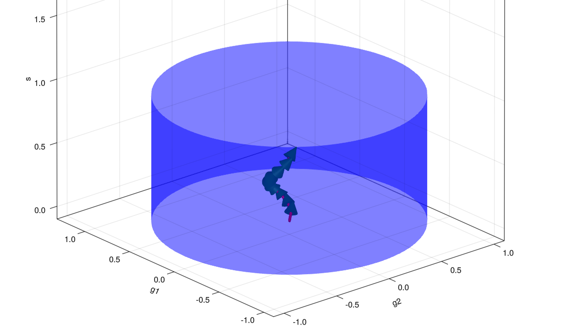
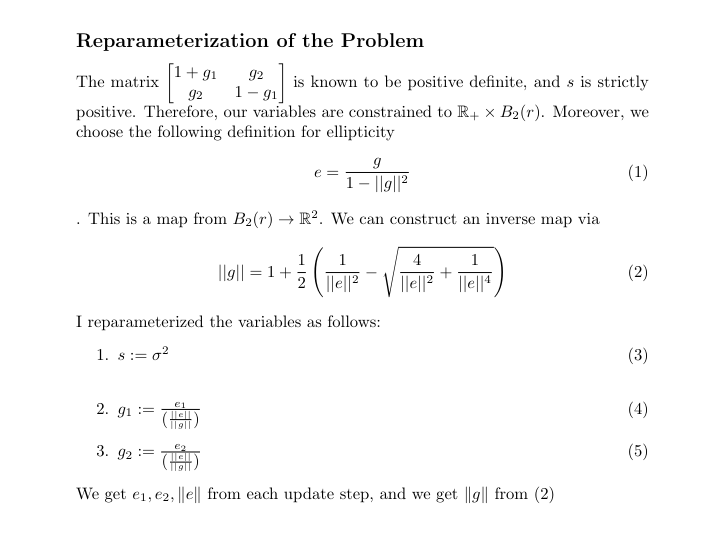
ShOpt.jl’s analytic profile fitting takes inspiration from a number of algorithms outside of astronomy, notably SE-Sync, an algorithm that solves the robotic mapping problem by considering the manifold properties of the data. With sufficiently clean data, the SE-Sync algorithm will descend to a global minimum constrained to the manifold \(SE(d)^n / SE(d)\). Following suit, we are able to put a constraint on the solutions we obtain to \([s, g_1, g_2]\) to a manifold. The solution space to \([s, g_1, g_2]\) is constrained to the manifold \(B_2(r) \times \mathbb{R}_{+}\). The existence of the constraint on shear is well known; nevertheless, the parameter estimation task is usually framed as an unconstrained problem.
Path to [s, g_1, g_2] through cylindrical constraint.
Pixel Grid Fits
PCA Mode
We used the first n weights of a Principal Component Analysis and use that to construct our PSF in addition to a smoothing kernel to account for aliasing
Autoencoder Mode
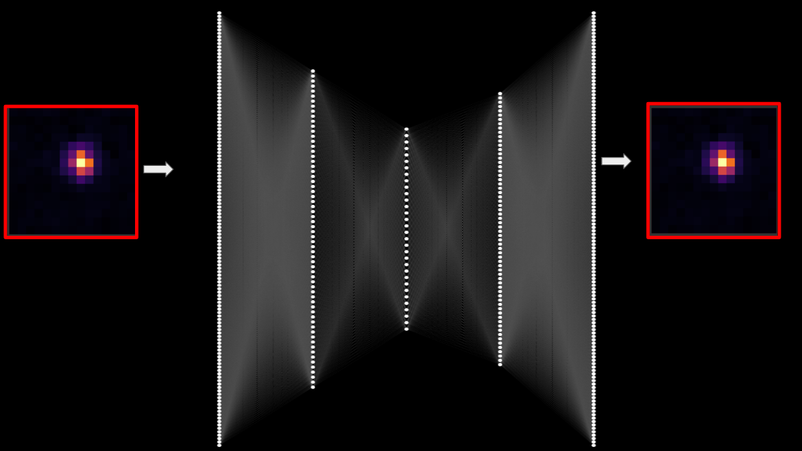
For doing Pixel Grid Fits we use an autoencoder model to reconstruct the Star
PCA mode
function pca_image(image, ncomponents)
  #Load img Matrix
  img_matrix = image

  # Perform PCA
  M = fit(PCA, img_matrix; maxoutdim=ncomponents)

  # Transform the image into the PCA space
  transformed = MultivariateStats.transform(M, img_matrix)

  # Reconstruct the image
  reconstructed = reconstruct(M, transformed)

  # Reshape the image back to its original shape
  reconstructed_image = reshape(reconstructed, size(img_matrix)...)
end
Autoencoder mode
# Encoder
encoder = Chain(
                Dense(r*c, 128, leakyrelu),
                Dense(128, 64, leakyrelu),
                Dense(64, 32, leakyrelu),
               )
#Decoder
decoder = Chain(
                Dense(32, 64, leakyrelu),
                Dense(64, 128, leakyrelu),
                Dense(128, r*c, tanh),
               )
#Full autoencoder
autoencoder = Chain(encoder, decoder)

#x_hat = autoencoder(x)
loss(x) = mse(autoencoder(x), x)

# Define the optimizer
optimizer = ADAM()
Interpolation Across the Field of View
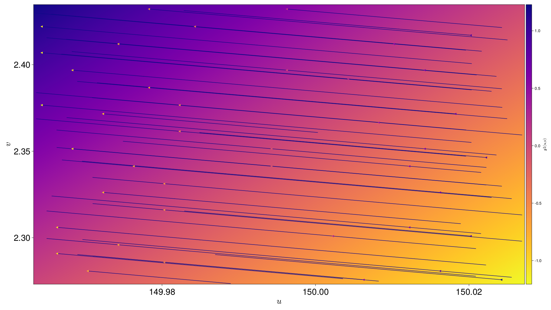
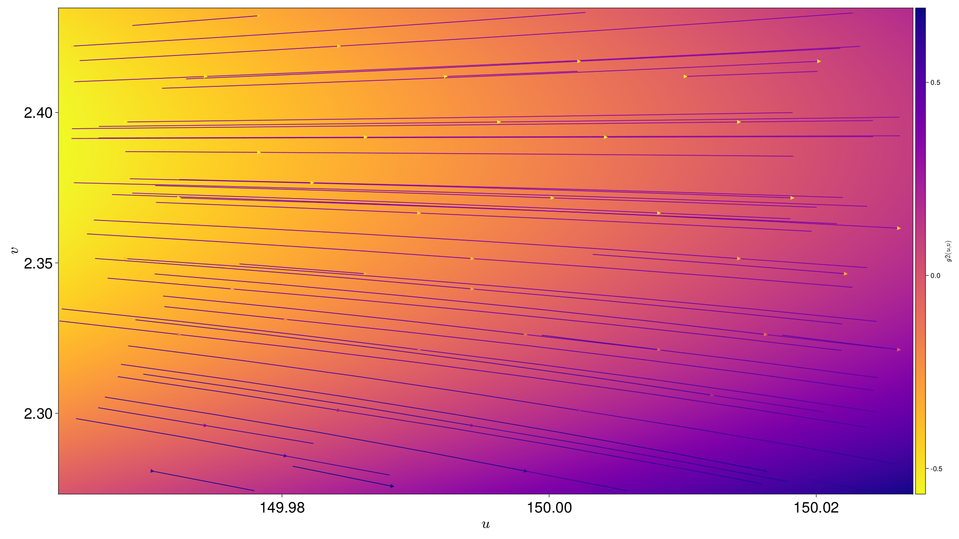
[s, g1, g2] are all interpolated across the field of view. Each Pixel is also given an interpolation across the field of view for an nth degree polynomial in (u,v), where n is supplied by the user
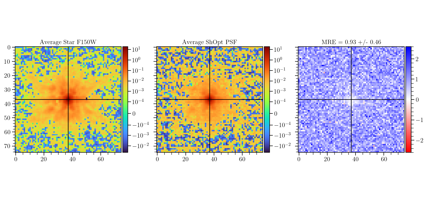 The plot on the left shows the average cutout of all stars in a supplied catalog. The plot in the middle shows the average point spread function model for each star. The plot on the right show s the average normalized error between the observed star cutouts and the point spread function model.
Inputs and Outputs
Currently, the inputs are JWST Point Spread Functions source catalogs. The current outputs are images of these Point Spread Functions, Learned Analytic Fits, Learned Pixel Grid Fits, Residual Maps, Loss versus iteration charts, and p-value statisitcs. Not all functionality is working in its current state. Planned functionality for more Shear checkplots.
Inputs
| Image | Description |
|---|---|
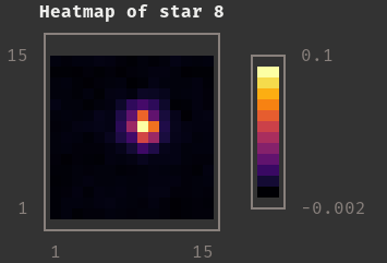 |
Star Taken From Input Catalog |
| shopt.yml | Config File for Tunable Parameters |
| * starcat.fits | Star Catalog to take vignets from |
Outputs
| Image | Description |
|---|---|
| summary.shopt | Fits File containing summary statistics and information to reconstruct the PSF |
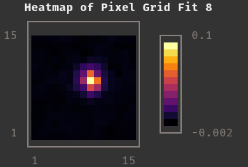 |
Pixel Grid Fit for the Star Above |
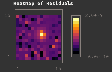 |
Residual Map for Above Model and Fit |
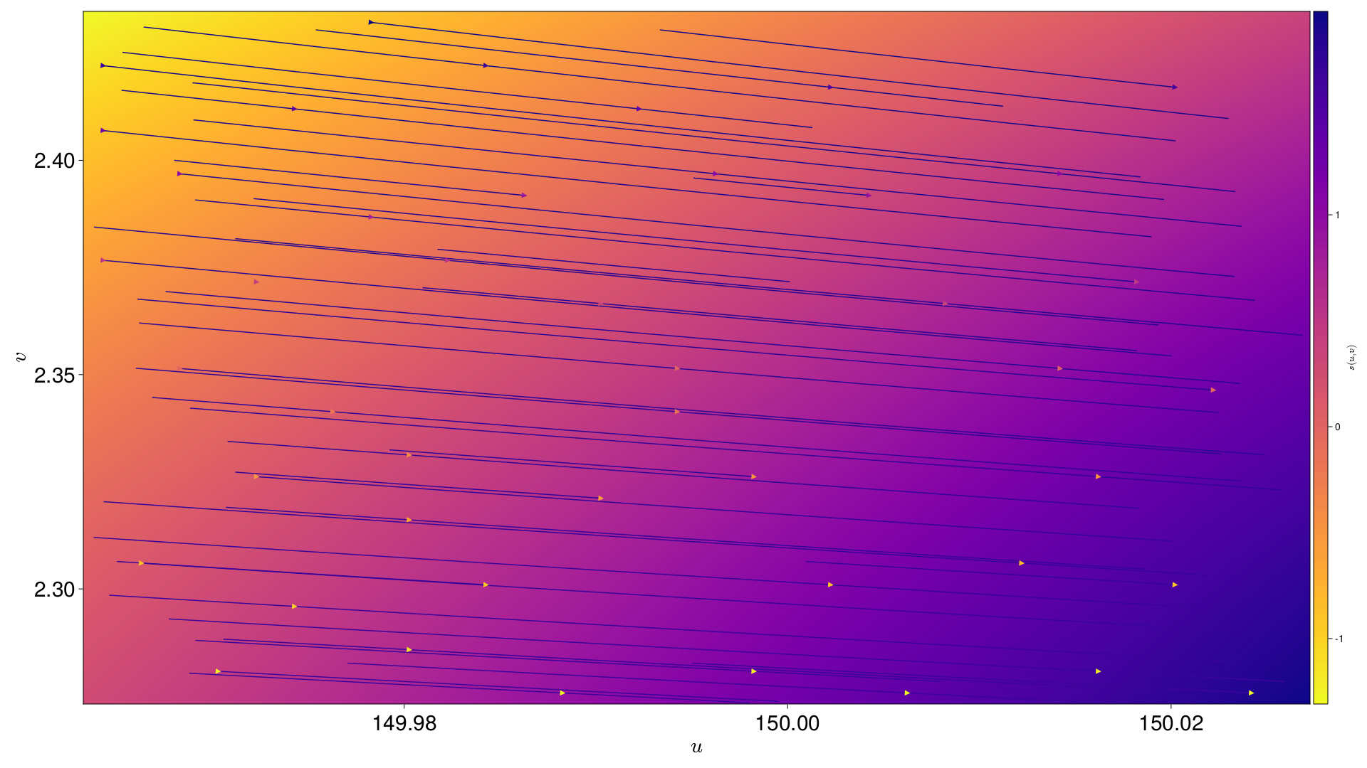 |
s varying across the field of view |
 |
g1 varying across the field of view |
 |
g2 varying across the field of view |
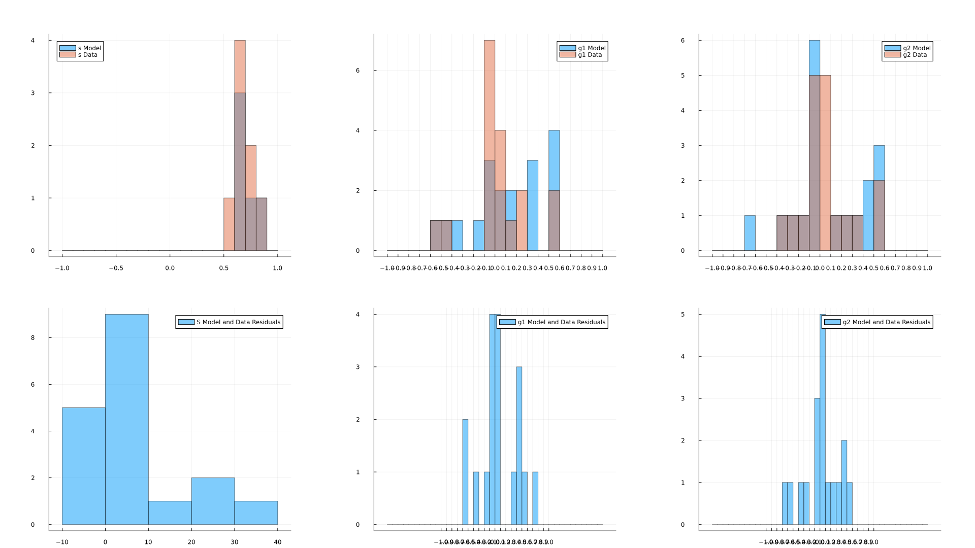 |
Histogram for learned profiles for each star in an analytic fit with their residuals |
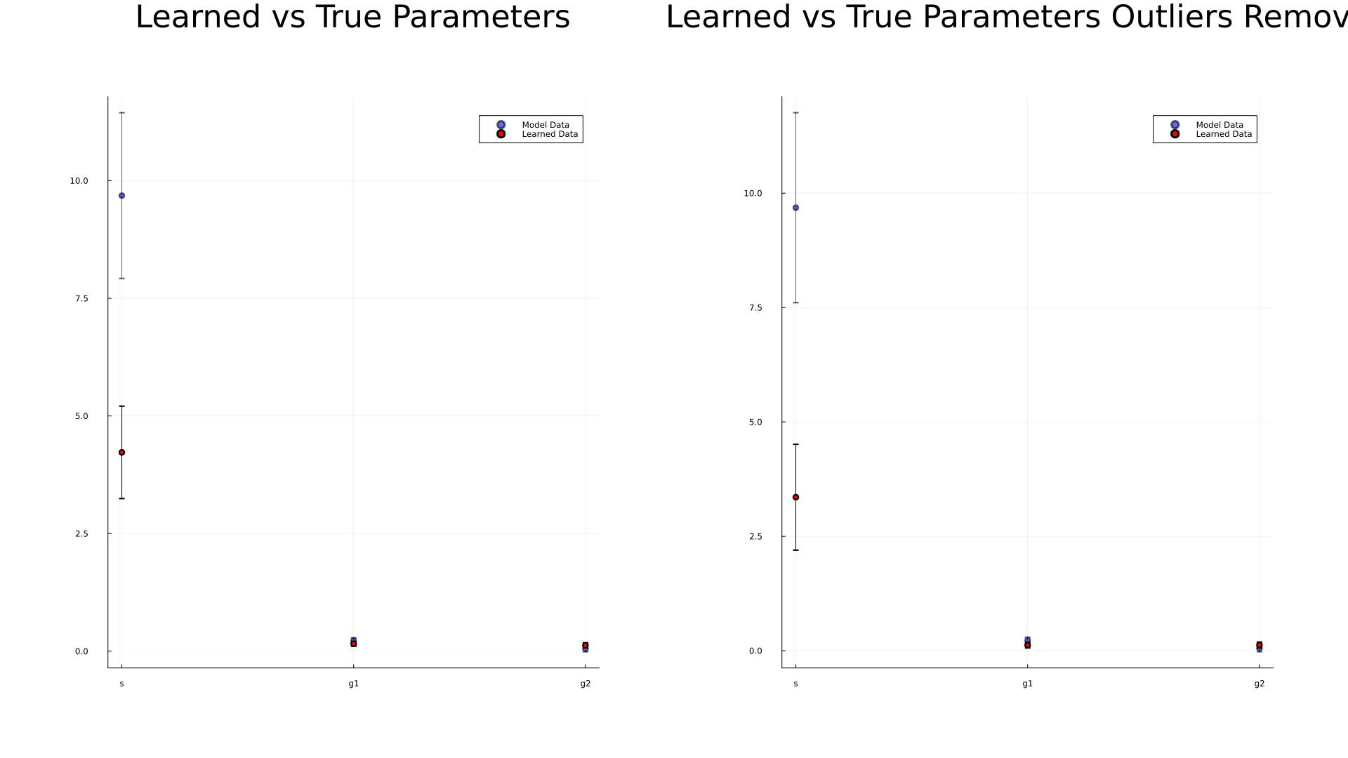 |
Same data recorded as a scatterplot with and without outliers removed and with error bars |
NB: This is not a comprehensive list, only a few cechkplots are presented. See the shopt.yml to configure which plots you want to see and save!
Running
Command
To run shopt.jl
First use Source Extractor to create a catalog for ShOpt to accept and save this catalog in the appropriate directory
Run julia shopt.jl [configdir] [outdir] [catalog]
There is also a shell script that runs this command so that the user may call shopt from a larger program they are running
Dependencies
Not all of these will be strictly necessary depending on the checkplots you produce, but for full functionality of ShOpt the following are necessary. Source Extractor (or Source Extractor ++) is also not a strict dependency, but in practice one will inevitably install to generate a catalog.
| Julia | Python | Binaries | Julia | Julia |
|---|---|---|---|---|
| Plots | matplotlib | SEx | ProgressBars | BenchmarkTools |
| ForwardDiff | astropy | UnicodePlots | Measures | |
| LinearAlgebra | numpy | CSV | Dates | |
| Random | FFTW | YAML | ||
| Distributions | Images | CairoMakie | ||
| SpecialFunctions | ImageFiltering | Flux | ||
| Optim | DataFrames | QuadGK | ||
| IterativeSolvers | PyCall | Statistics |
Set Up
Start by cloning this repository. There are future plans to release ShOpt onto a julia package repository, but for now the user needs these files contents.
The dependencies can be installed in the Julia REPL. For example:
import Pkg; Pkg.add("PyCall")
We also provide dependencies.jl, which you can run to download all of the Julia libraries automatically by reading in the imports.txt file. Simply run julia dependencies.jl in the command line. For the three python requirements, you can similarly run python dependenciesPy.py. We also have a project enviornment for the Julia packages in the folder shopt_env. It would be straightforward to add the line activate(“shopt_env”) to the first line of shopt.jl to read in this environment. Note that Pycall would have to be built within this environment in some of the next steps.
For some functionality we need to use wrappers for Python code, such as reading in fits files or converting (x,y) -> (u,v). Thus, we need to use certain Python libraries. Thankfully, the setup for this is still pretty straightfoward. We use PyCall to run these snippets.
There are four different methods to get Julia and Python to interopt nicely. We provide all of them as some of these methods play better with different systems.
First install the required Python libraries via pip (which is what dependenciesPy.py does). Now, for method 1, invoke the following in the julia REPL:
using PyCall
ENV["PYTHON"] = "/path_desired_python_directory/python_executable"; import Pkg; Pkg.build("PyCall")
pyimport("astropy")
It is important that the command pyimport(“astropy”) should be run after re-loading the Julia REPL.
Method 2. If you have a Conda Enviornment setup, you may find it easier to run
using PyCall
pyimport_conda("astropy", "ap") #ap is my choice of name and astropy is what I am importing from my conda Enviornment
Method 3. julia also has a way of working with conda directly. Note that julia will create its own conda enviornment to read from.
using Conda
Conda.add("astropy", :my_env) #my conda enviornment is named my_env
You may also do using Conda; Conda.add("astropy", "/path/to/directory") or using Conda; Conda.add("astropy", "/path/to/directory"; channel="anaconda")
Method 4. On the off chance that none of these works, a final method may look like the following
using PyCall
run(`$(PyCall.python) -m pip install --upgrade cython`)
run(`$(PyCall.python) -m pip install astropy`)
After the file contents are downloaded the user can run julia shopt.jl [configdir] [outdir] [catalog] as stated above. Alternatively, they can run the shellscript that calls shopt in whatever program they are working with to create their catalog. For example, in a julia program you may use run(`./runshopt.sh [configdir] [outdir] [catalog]`)
Multithreading
Before running, we recommend that users run export JULIA_NUM_THREADS=4 on Unix machines set JULIA_NUM_THREADS=4 . By default Julia will run the program on a single thread, but the polynomial interpolation step is inherently parallelizable. The program is set to use all of threads available to it. You may do more than 4, just be cautious about what your system can provide and when you start getting dimminishing returns.
Testing
To test that everything works, running the dependencies.jl should test that everything is installed correctly in addition to downloading. Running
pyimport("astropy")
pyimport("matplotlib")
pyimport("numpy")
in the Julia REPL should ensure that Julia and Python are interopping correctly.
Additionally, in the Julia REPL, we may write
using Base.Threads
nthreads()
to make sure we are using 4 or more threads. The TutorialNotebook.ipynb will walk you through and test all of the functionality of the program.
Program Architecture
TutorialNotebook.ipynb
Run ShOpt inside of a Jupyter Notebook and learn both how to run the program and how to reconstruct the PSF
shopt.jl
A runner script for all functions in this software
dataPreprocessing.jl
A wrapper for python code to handle fits files and dedicated file to deal with data cleaning
dataOutprocessing.jl
Convert data into a summary.shopt file. Access this data with reader.jl. Produces some additional python plots.
reader.jl
Get Point Spread Functions at an arbitrary (u,v) by reading in a summary.shopt file
plot.jl
A dedicated file to handle all plotting
radialProfiles.jl
Contains analytic profiles such as a Gaussian Fit and a kolmogorov fit
analyticLBFGS.jl
Provides the necessary arguments (cost function and gradient) to the optimize function for analytic fits
pixelGridAutoencoder.jl
Houses the function defining the autoencoder and other machine learning functions supplied to Flux’s training call
interpolate.jl
For Point Spread Functions that vary across the Field of View, interpolate.jl will fit a nth degree polynomial in u and v to show how each of the pixel grid parameters change across the (u,v) plane
outliers.jl
Contains functions for identifying and removing outliers from a list
powerSpectrum.jl
Computes the power spectra for a circle of radius k, called iteratively to plot P(k) / k
kaisserSquires.jl
Computes the Kaisser-Squires array to be plotted
runshopt.sh
A shell script for running Shopt. Available so that users can run a terminal command in whatever program they are writing to run shopt.
LICENSE
MIT LICENSE
README.md
User guide, Dependencies, etc.
index.md
For official website
_config.yml
Also for official website
imports.txt
List of Julia Libraries used in the program
packages.txt
List of Python Libraries used in the program
dependencies.jl
Download all of the imports from imports.txt automatically
dependenciesPy.py
Download all of the imports from packages.txt automatically
Config / YAML Information
saveYaml
- Set
trueif you want to save the YAML to the output directory for future reference, set tofalseotherwise
NNparams
- epochs
- Set the Maximum Number of training epochs should the model never reach the minimum gradient of the loss function. Set to
1000by default
- Set the Maximum Number of training epochs should the model never reach the minimum gradient of the loss function. Set to
- minGradientPixel
- A stopping gradient of the loss function for a pixel grid fit. Set to
1e-6by default
- A stopping gradient of the loss function for a pixel grid fit. Set to
AnalyticFitParams
- minGradientAnalyticModel
- A stopping gradient of the loss function for an analytic profile fit for input star vignets from a catalog. Set to
1e-6by default
- A stopping gradient of the loss function for an analytic profile fit for input star vignets from a catalog. Set to
- minGradientAnalyticLearned
- A stopping gradient of the loss function for an analytic profile fit for stars learned by a pixel grid fit. Set to
1e-6by default
- A stopping gradient of the loss function for an analytic profile fit for stars learned by a pixel grid fit. Set to
- analyticFitStampSize
- The box size for the subset of your stamp (see stamp size) you wish to use for analytic profile fitting. Ensure to specify this to be smaller than the stamp size of the vignets themselves. Set to
64by default, therefore fitting an analytic profile to the middle64 x 64pixels of the stamp.
- The box size for the subset of your stamp (see stamp size) you wish to use for analytic profile fitting. Ensure to specify this to be smaller than the stamp size of the vignets themselves. Set to
dataProcessing
- SnRPercentile
- Supply a float that represents the percentile below which stars will be filtered by on the basis of signal to noise ratio. Set to
0.33by default
- Supply a float that represents the percentile below which stars will be filtered by on the basis of signal to noise ratio. Set to
- sUpperBound
- Stars fit with an analytic profile are filtered out if their
sexceeds this upper bound. Set to1by default
- Stars fit with an analytic profile are filtered out if their
- sLowerBound
- Stars fit with an analytic profile are filtered out if their
sfalls beneath this lower bound. Set to0.075by default
- Stars fit with an analytic profile are filtered out if their
plots
- Set true to plot and save a given figure, false otherwise
polynomialDegree
- The degree of the polynomial used to interpolate each pixel in the stamp across the field of view. Set to
3by default
stampSize
- The size of the vignet for which use wish to fit. Used interpolation for oversampling and a simple crop for undersampling. Set to
131by default to fit and interpolate131 x 131pixels
training_ratio
- Before doing a polynomial interpolation, the remaining stars will be divided into training and validation stars based off of this float. Set to
0.8by default, indicating 80% training stars 20% validation stars
CommentsOnRun
- This is Where You Can Leave Comments or Notes To Self on the Run! Could be very useful if you save the yaml file with each run
How to Contribute
Do one of the following:
- Contact berman.ed@northeastern.edu
- Fork this repository or submit a pull request
If you would like to report an issue or problem please raise an issue on this repository. If you would like to seek support, again see berman.ed@northeastern.edu .
Known Issues and Enhancements
- We are working on more configurability in the YAML for a smoother user experience, however, everything in this repository is functional and ready to work out of the box
- We are working on a chisq pixel grid fit mode. Right now the gain value g is hardcoded for chi square pixel grid fits
Contributors
- Edward Berman
- Jacqueline McCleary
With help from collaborators at COSMOS-Web: The JWST Cosmic Origins Survey
Further Acknowledgements
- The Northeastern Cosmology Group for Their Continued Support and Guidance
- The Northeastern Physics Department and Northeastern Undergraduate Research and Fellowships, for making this project possible with funding from the Northeastern Physics Research Co-Op Fellowship and PEAK Ascent Award respectively
- David Rosen, who gave valuable input in the early stages of this project and during his course Math 7223, Riemannian Optimization
- The COSMOS Web Collaboration for providing data from the James Webb Space Telescope and internal feedback
Cite
Citation for the current Astronomical Journal (AJ) preprint:
@article{berman2024efficientpsfmodelingshoptjl,
doi = {10.3847/1538-3881/ad6a0f},
url = {https://dx.doi.org/10.3847/1538-3881/ad6a0f},
year = {2024},
month = {sep},
publisher = {The American Astronomical Society},
volume = {168},
number = {4},
pages = {174},
author = {Edward M. Berman and Jacqueline E. McCleary and Anton M. Koekemoer and Maximilien Franco and Nicole E. Drakos and Daizhong Liu and James W. Nightingale and Marko Shuntov and Diana Scognamiglio and Richard Massey and Guillaume Mahler and Henry Joy McCracken and Brant E. Robertson and Andreas L. Faisst and Caitlin M. Casey and Jeyhan S. Kartaltepe and COSMOS-Web: The JWST Cosmic Origins Survey},
title = {Efficient Point-spread Function Modeling with ShOpt.jl: A Point-spread Function Benchmarking Study with JWST NIRCam Imaging},
journal = {The Astronomical Journal},
abstract = {With their high angular resolutions of 30–100 mas, large fields of view, and complex optical systems, imagers on next-generation optical/near-infrared space observatories, such as the Near-Infrared Camera (NIRCam) on the James Webb Space Telescope, present new opportunities for science and also new challenges for empirical point-spread function (PSF) characterization. In this context, we introduce ShOpt, a new PSF fitting tool developed in Julia and designed to bridge the advanced features of PSFs in the full field of view (PIFF) with the computational efficiency of PSF Extractor (PSFEx). Along with ShOpt, we propose a suite of nonparametric statistics suitable for evaluating PSF fit quality in space-based imaging. Our study benchmarks ShOpt against the established PSF fitters PSFEx and PIFF using real and simulated COSMOS-Web Survey imaging. We assess their respective PSF model fidelity with our proposed diagnostic statistics and investigate their computational efficiencies, focusing on their processing speed relative to the complexity and size of the PSF models. We find that ShOpt can already achieve PSF model fidelity comparable to PSFEx and PIFF while maintaining competitive processing speeds, constructing PSF models for large NIRCam mosaics within minutes.}
}
Citation for the Journal of Open Source Software (JOSS) paper:
@article{Berman2024, doi = {10.21105/joss.06144}, url = {https://doi.org/10.21105/joss.06144}, year = {2024}, publisher = {The Open Journal}, volume = {9}, number = {100}, pages = {6144}, author = {Edward Berman and Jacqueline McCleary}, title = {ShOpt.jl: A Julia Package for Empirical Point Spread Function Characterization of JWST NIRCam Data}, journal = {Journal of Open Source Software} }

